Since the 5th century BC, when Pheidippides ran from Marathon to Athens to deliver the news of a battle victory; running 42.195km has remained the pinnacle of endurance activities.
Marathons are a great metaphor for careers, building businesses and winning in life. And the common phrase you will often hear is “Investing is a marathon not a sprint”. But how many people who use this line have actually run one? As both a marathon runner and a long-term investor here are ten of my favourite insights on the parallel between the two:
You don’t run 42km once. You run one kilometre forty-two times. Insight: Break the big task up into smaller goals and SIPs are the best way to do this.
A marathon is a 10km race with a 32km warmup. Insight: Compounding is back ended.
Every uphill has a downhill. Insight: In markets, things are never as good or as bad as they seem.
To finish first, you must first finish Insight: It doesn’t matter how late you started, how little you are saving or how far away your financial goal is. Just keep going!
It never gets easier, you only get faster Insight: Progress is the essence of life. Keep growing and raising your ambition.
You only see the runners in front of you, never those behind you Insight: Appreciate everything you have and how far you have come in life. Gratitude and contentment are pillars of long-term compounding.
The hardest part is not finishing, it is believing you can finish Insight: Self-belief is your greatest source of strength. And focus on the present and only on the present.
A marathon is not run on the road. It is run in the six inches between your ears. Insight: Equanimity is the secret to success in long-term investing.
For every minute you gain on the first half, you will give back three in the second half. Insight: Stay patient and stick to your plan. There are no shortcuts to getting rich.
It takes a team to run a marathon alone Insight: Acknowledge and celebrate the role your financial advisor, family and friends play in your financial success.
Have you thought about the PRC rating in liquid funds? Do you know why it matters and what the matrix represents for these funds?
The PRC (Potential Risk Class) matrix, introduced by SEBI, requires debt funds to disclose the maximum level of risk they intend to take in the future based on their current and future investments.
This matrix evaluates two major risks that debt mutual funds are exposed to:
1. Credit Risk – the risk that the issuer of security may default.
2. Interest Rate Risk – the risk of the security’s value fluctuating due to changes in interest rates.
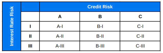
The position of the debt scheme in the matrix shall be displayed by the AMCs by this matrix. Here is have a look at the matrix –
Let me interpret it for you, the Rows I,II and III represent the interest rate risk a fund can take with Row I being the relatively low risk (Macaulay Duration ≤ 1 year), Row II being the moderate risk (Row II: Moderate risk (Macaulay Duration ≤ 3 years) and Row III being the relatively high interest rate risk (Any Macaulay Duration). In the case of liquid funds, investments are restricted to securities with maturity up to 91 days. Because of this short duration, interest rate risk is minimal. Therefore, liquid funds are always placed in the Row “I” category, indicating relatively low-interest rate risk.
However, the PRC rating still matters because liquid funds can differ in credit risk, depending on the type of short-term instruments they choose—ranging from very high-quality (AAA rated) securities to slightly lower-rated ones. Category ranges from columns A to C represents the credit risk a fund is willing to take, Column A being the lowest and Column C being the highest.
SEBI has assigned a Credit Risk Value (CRV) to different categories of debt securities. The higher the CRV, the lower the potential credit risk—and vice versa.
· Government securities (G-Secs), State development loans/Treasury Bills/ Repo on Government Securities/TREPS / Cash carry a CRV of 13
· AAA-rated securities have a CRV of 12
· AA+ securities have a CRV of 11
· AA securities have a CRV of 10 and so on
Classification based on the weighted average CRV of a fund’s portfolio:
· CRV ≥ 12 → Classified as “A” class (relatively low credit risk)
· CRV of 10–11 → Classified as “B” class (moderate credit risk)
· CRV < 10 → Classified as “C” class (relatively high credit risk)
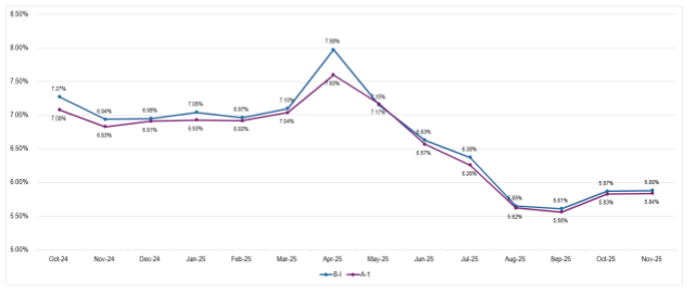
Although moderate credit-risk funds should theoretically outperform low credit-risk funds on a risk-adjusted basis, the performance differential has meaningfully narrowed over the past one year. This trend has been influenced by improved market flows, compression in credit spreads, and a strategic tilt among fund managers toward lower credit-risk instruments.
Median Rolling returns of PRC A-I vs B-I Liquid Funds
Source: ICRAMFI360, PPFAS Research
The spread between median rolling returns of A-I and B-I rated liquid funds has been reduced over the past year with better liquidity conditions since April 2025. A fund that takes higher credit risk may offer slightly higher returns but with increased potential volatility or credit events. Since liquid funds are designed primarily for short-term goals and emergency requirements, safety and liquidity should be preferred over returns.
Disclaimer – The views are personal. Macaulay Duration (Duration) measures the price volatility of fixed income securities. It is often used in the comparison of interest rate risk between securities with different coupons and different maturities. It is defined as the weighted average time to cash flows of a bond where the weights are nothing, but the present value of the cash flows themselves. It is expressed in years/days. The duration of a fixed income security is always shorter than its term to maturity, except in the case of zero-coupon securities where they are the same. The Potential Risk Class (PRC) matrix, mandated by SEBI, discloses the maximum interest rate and credit risk a debt scheme may assume. PRC classification provides transparency on permissible risk boundaries but does not guarantee safety, liquidity, or returns. Past performance, including the mentioned narrowing of return differentials between A‑I and B‑I liquid funds, is not indicative of future results. Investors should evaluate their objectives and risk tolerance and consult the respective Scheme Information Document (SID), Key Information Memorandum (KIM), and professional advisors before investing.
Mutual Fund investments are subject to market risks, read all scheme related documents carefully.
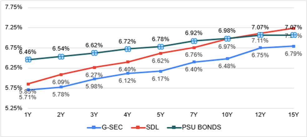
Corporate bond yields attracted strong investor interest up to July 2025, with record-high issuances being comfortably absorbed by the market. Spreads remained attractive relative to State Development Loans (SDLs). Backed by the RBI’s liquidity easing measures and a cumulative 100 bps of rate cuts in CY2025, overall liquidity conditions have turned comfortable. Corporate bonds continued to offer appealing spreads as investors sought to lock in higher yields amid expectations of further rate declines. Notably, the corporate bond curve, which had remained inverted last year amid liquidity deficit conditions, has now steepened in line with improving market dynamics.
Bond Yield Curve (31st July,2025) Source: CCIL (Yields are annualized)
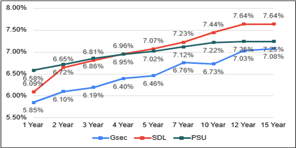
Following the August 2025 monetary policy meeting, a more cautious tone has emerged. Fiscal concerns linked to GST reforms, tariff-related announcements, and subdued bank demand have driven yields higher across G-Secs and SDLs. Elevated state borrowing has also added pressure, with issuances in FY25 (up to 15 August 2025) rising to Rs 3.80 lakh crore compared to Rs 2.53 lakh crore in the same period of FY24. As a result, SDL spreads over G-Secs have widened sharply to 70–80 bps, well above their usual 45–50 bps range. Lower participation from insurance and pension funds—particularly at the longer end, where they typically dominate—has further contributed to the steepening.
In contrast, corporate bond issuances remained muted in August 2025 as issuers refrained from locking in debt at elevated interest rates. A few attempted issues were eventually withdrawn amid higher investor bid expectations. The combination of elevated SDL yields and subdued corporate supply has driven a sharp compression in AAA PSU corporate bond spreads over the past month. While the PSU corporate bond yield curve remains steep, spreads have narrowed considerably—turning unattractive beyond the 2–3-year segment, where they have even slipped into negative territory. The government bond yield curve including SDLs has now turned more attractive, with unusual spreads emerging from the recent steepening. However, given these unusual circumstances, the expectation is that the RBI to intervene and stabilize the market through appropriate measures.
Yield Curve (26th August ,2025) Source: CCIL (Yields are annualized)
In September’s FOF, I gave a presentation on the Opportunity and Challenges in Smallcap Investing. A recurrent question post the presentation was about how Smallcaps which have become Largecaps have generated a lot of wealth and consequently doesn’t it make Smallcaps attractive? Here’s a thought many share: When we look at the list of past multibaggers, we often find that many of those stocks started as Smallcaps. This leads some to infer that the probability of a smallcap becoming a multibagger is very high.
What does the actual data tell us? Let’s define a stock that offers a 30% Compound Annual Growth Rate (CAGR) over five years as a ‘multibagger’. Analyzing past data (from 2013 to 2018) from the top 500 stocks, we find that there’s an 11% chance of any stock becoming a multibagger. Focusing only on Smallcaps, that probability rises slightly to 13%. In other words, out of 250 Smallcap stocks, only about 33 might deliver such returns. Furthermore, there’s a 16% chance of a Smallcap stock declining by 50% over five years, compared to 14% for the broader stock group. This data suggests we might be greatly overestimating the allure of Smallcaps.
But the interesting question is why do we overestimate these odds? The answer lies in a fallacy most of us fall prey to – Base Rate Fallacy. What appears to us a high probability phenomenon actually turns out to be a low probability phenomenon.
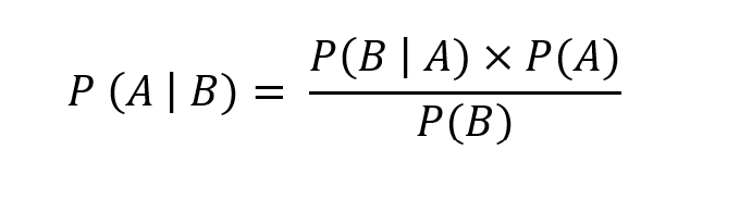
To understand Base Rates, we need to understand Bayes Theorem; a cornerstone of probability theory. And for that we need some notation. At first glance, the mathematical notation may seem daunting, but trust me, it’s quite simple and intuitive.
P(A) : Probability of event A occurring P(A | B) : Probability of event A occuring, given that B has occurred. In other words, if we know that B is true, then what is the probability of A
Now, Bayes rule states that:
Translated to plain terms: If you want to know the probability of A happening given that B has happened – P(A|B), you can figure it out by looking at:
P(B|A) – How often B happens when A happens, P(A) – The overall likelihood of A happening on its own, and P(B) – Dividing those by how often B happens in general.”
A common error is to confuse P(A|B) with P(B|A). This error is also called the Inverse Probability error
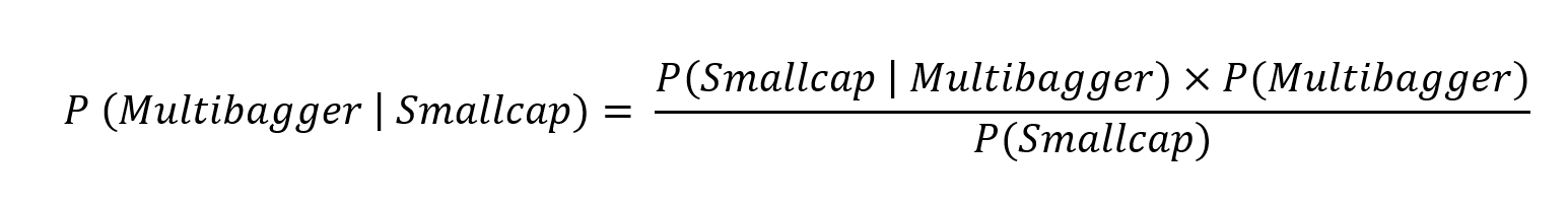
Now, with this context let’s evaluate the probability of smallcaps turning to large caps. So let’s put this in notation. We know a stock is a multibagger and we believe many of these are smallcaps. When we look at past multibaggers we find that 60% of the multibaggers were smallcaps.
P (Smallcap | Multibagger) = 0.6
It might be tempting to take this 60% as the probability that a Small Cap would become a Multbagger. But as we will see that would be a major error in estimating probabilities. When you think about it, what we really want to know is if a given stock is a smallcap, what is the probability that it will become a multibagger i.e. P (Multibagger | Smallcap)
By Bayes Theorem :
Of the top 500 stocks, half are Smallcap. So we know the probability of smallcap – P(Smallcap) = 0.5
Also, of all the listed stocks we found that approximately 11% of stocks become multibaggers; so P(Multibagger) = 0.11
Now, we have the required probabilities to calculate the probability we want
P (Multibagger | Smallcap) = (0.6 x 0.11)/0.5 = 0.13 i.e. 13%
The reason for this low probability is that the overall base rate for a stock becoming a multibagger – P(Multibagger) is extremely low (11%) and that number dominates the probability of a smallcap becoming a multibagger. Our intuition makes us focus on P(Smallcap | Multibagger) but the number that influences the end probability much more is P(Multibagger). You can try different assumptions for P(Smallcap|Multibagger) and P(Multibagger) in the formula and what you will find is that so long as P(Multibagger) is very low, the end probability will also be low.
Once you understand and appreciate inverse probabilities, you will see them everywhere. For example: many studies and books focus on very successful companies and try to identify the traits common to them. Again this is actually an Inverse Probability problem and prone to Base Rate fallacy. By starting with a list of very successful companies and then identifying a common trait, we are finding P(Trait | Success). What we are actually interested in is P(Success | Trait) i.e. if a company has a given Trait then what is the probability that it will be successful.
How can we mitigate this fallacy? When probabilistic judgements, especially for low probability events, we need to take a step back and ask ourselves whether the Probability we have calculated or assumed is what is relevant to the decision or have we estimated an Inverse probability where we need to account for base rates. By ensuring that we critically evaluate the information at hand and avoid jumping to conclusions based on intuition or selective data, we can make more informed and rational decisions.
There is a saying – “When the student is ready, the master appears, but when the student is truly ready the master disappears.”
Learn from Others
Those who do not have experience, learn by watching & studying others. It’s a valuable part of our development. This is exactly how kids learn how to speak or pick up a vocabulary and an accent by imitating and watching their parents. Mirroring others is an established form of learning.